MOTION SENSOR
Elizabeth Beck
Lab Partner: Allison Butrie
18 March 2014
Lab Partner: Allison Butrie
18 March 2014
Purpose
In this lab we hope to discover relationships between graphs of motion and the equations that describe them.
Theory
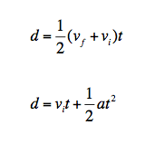
The kinematic equations used in his experiment are:
Acceleration is constant with all the kinematic equations.
Experimental Technique
|
Materials Used:
|
|
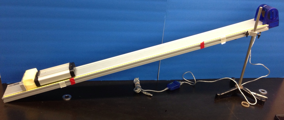
Procedure:
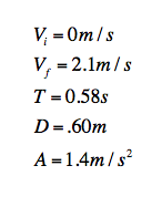
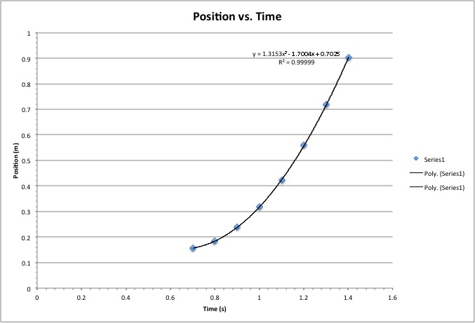
To start this experiment first I assembled the inclined plane and hooked up the motion sensor. Then I marked the distance I would be measuring with strips of red tape. The tape was at 90cm and 30 cm, making the total distance measured 60cm. I converted the 60cm to 0.60m. Then I set up the Mac and took a video of the cart rolling down the inclined plane to find the exact time it took for the cart to travel the distance I had marked, which is 0.58s. Then we used the information we collected to find the five kinematic values. To make a graphical representation of the equations I turned on the motion sensor and collected the data from the corresponding program. This gave us a position versus time graph. Then we used equations listed below to find and graph the velocity and acceleration of the cart. Finally we used the kinematic values from earlier to check if the graphs followed the equations.
To start this experiment first I assembled the inclined plane and hooked up the motion sensor. Then I marked the distance I would be measuring with strips of red tape. The tape was at 90cm and 30 cm, making the total distance measured 60cm. I converted the 60cm to 0.60m. Then I set up the Mac and took a video of the cart rolling down the inclined plane to find the exact time it took for the cart to travel the distance I had marked, which is 0.58s. Then we used the information we collected to find the five kinematic values. To make a graphical representation of the equations I turned on the motion sensor and collected the data from the corresponding program. This gave us a position versus time graph. Then we used equations listed below to find and graph the velocity and acceleration of the cart. Finally we used the kinematic values from earlier to check if the graphs followed the equations.
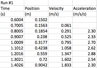
Data
|
|
Analysis
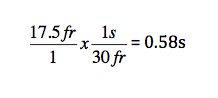
To find the time, I used the video and counted the number of frames it took the cart to travel .60m which was 17.5 frames. Then I converted it to seconds with this equation:
|
To find the final velocity I used the equation:
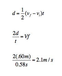
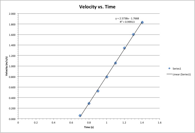
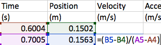
To find the velocity of the points on the graph I used the equation:
|
To find the acceleration I used the equation:
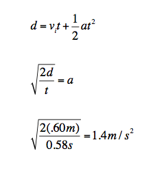
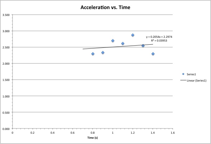
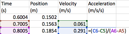
To find the acceleration of the points on the graph I used the equation:
|
Conclusion
In this lab our goal was to see if the our graphical analysis matched up with the kinematic equations. First, measured the initial velocity, time and distance from the cart moving on the inclined plane. I used the kinematic equations to find the acceleration and final velocity. The equations mostly matched up with the graphs except for the acceleration. In theory, acceleration would be constant and therefore linear. Since there are only a few points graphed the points are less linear but still fall in close proximity to the trend line.
